Let's go with 100Hz first because it feels easier to debug to me.
Going Deep (Low Level)
It might be OK for 100Hz, but we can't be using digitalWrite or any of that high level crap for fast signal generation, like, say, 100kHz. We need to go deep and mess with with literal processor registers among other embedded exclusive (TM) things. We need to do real hardware PWM to obtain a waveform that precise.
Details
The reactance formulae like $\frac{1}{2\pi f C}$ are for a pure sinusoidal waveform. The square wave coming from the microcontroller is not. We'll be dealing with this problem later on but for the time being it is good enough. This is because a square wave is an infinite Fourier sum of sine waves, and the first harmonic is a sine wave with the same frequency as the original wave.
There is a crystal on the PCB (curved cylinder looking flat thing) that is oscillating at a frequency of 16MHz. Every tick on the crystal clocks a timer (Timer 1 on Nano) that is essentially a 16-bit binary counter. This timer supports a CTC mode (Clear Timer on Compare Match) where you can tell it after what number to reset (TOP value). There is also something called a prescaler that is a hardware counter that slows down the counting rate of the oscillator by swallowing every tick except $n \cdot prescaler$.
So if you want a square wave of frequency $f$:
$$ f = \frac{16000000}{2 \cdot prescaler \cdot TOP} $$
The 2 is there because it takes two clock cycles to create one cycle of a square wave. The prescaler is like a gearbox for the oscillator: if you set it too low it will be really precise but the timer will overflow quite quickly; if you set it too high it won't be as precise but will support longer intervals (longer overflow time) For me prescaler = $8$ hasn't disappointed me.
On the Nano, pin 9 is one of the pins that is connected to Timer 1. The code looks like this:
#define SIGNAL_PIN 9
#define SENSE_PIN A0
#define SENSE_R 994
#define REFERENCE_V 4.49f

#define STRINGIFY(A) #A
#define SERIAL_PLOTTER_Y_BOUNDS(lower, upper) Serial.print("Min:" STRINGIFY(lower) ",Max:" STRINGIFY(upper) ",Value:")

void setup_timer() {
  pinMode(SIGNAL_PIN, OUTPUT);

  // Reset Timer 1 Control Registers
  TCCR1A = 0;
  TCCR1B = 0;
  TCNT1  = 0;

  // OC1A stands for "Output Compare Channel A" for Timer 1
  // Set the reset value. The TOP value is OCR1A + 1 because the counter is 0 indexed
  // TOP = 10000 so f = 16000000 / (2 * 8 * 10000) = 100 [Hz]
  OCR1A = 9999;

  // Set CTC mode (Clear Timer on Compare Match)
  TCCR1B |= (1 << WGM12);

  // 2. Set "Toggle OC1A on Compare Match"
  TCCR1A |= (1 << COM1A0);

  // 3. Set Prescaler to 8
  TCCR1B |= (1 << CS11);
}

void setup() {
  setup_timer();
  Serial.begin(115200);
}

float calculate_vcc(uint16_t count) {
  return ((float)count / 1023.0f) * REFERENCE_V;
}

void loop() {
  // Notice how we aren't multitasking here now?

  uint16_t count = analogRead(SENSE_PIN);
  float vcc = calculate_vcc(count);

  SERIAL_PLOTTER_Y_BOUNDS(0, REFERENCE_V);
  Serial.println(vcc);
}
This is a strictly electronical process with little to no software logic involved. Consequently with hardware PWM we spend close to 0% CPU usage for the switching. It is also clean and precise than the counter based method I used for logging in the previous chapter.
Upside Down
Hopefully you have realized that the circuitry insofar hasn't changed one bit since Zwitschenzeug by the way, but now we have to switch things up. We will to swap the resistor and capacitor to do low-side sensing. Essentially we will be measuring the voltage across the resistor ($V_{sense}$) instead of $V_{cap}$. We do this simply because measuring the circuit current $I$ (via the resistor) is the most difficult step in calculating the impedance from what I see, and we need all of the precision we got to do it. Putting the resistor first means we can measure the voltage across it directly ($V_{sense}$) without having to subtract it from the source voltage, which would've introduced another layer of uncertainty.
Details
Turns out the source voltage is a source of uncertainty in and of itself! I do fix a REFERENCE_V after literally measuring it with my multimeter, but the measured thing is the disconnected regulated voltage. At 100Hz (and beyond) there are tons of MOSFETs and all switching inside the MCU that are introducing their own voltage sags so it sort of "wobbles" around REFERENCE_V. I am not claiming I am building a Keysight Multimeter but it would be nice to deal with this extra layer of error. The solution is to look at the ground voltage which is -- from the definition of a potential difference -- always 0V! So by putting the resistor first, we don't have to subtract it from $V_{source}$ anymore, thereby eliminating that extra uncertainty from the source voltage. But now the burden of the extra voltage is on the cap, and we'll see later that calculating $Z$ involves both V's, so that uncertainty is going to be sneaking in no matter what. So why are we doing this? The answer is simply that it is more difficult to get accurate readings for the resistor compared to the capacitor, as stated above. A resistor has really sharp transients across it even at 100Hz so it is crucial that its readings are accurate enough. On the other hand, a capacitor literally smooths voltage (literally a low-pass filter) as we saw like two writeups ago, and that smooth voltage is much easier to detect by the ADC. By doing so we sort of optimize for the lowest uncertainty.
Now here comes the exciting part (at least for me): We can actually see that impedance is a real thing and not something made up by Big Electrical to lead people away from $V = IR$! Most importantly we can do it with a cheap multimeter that has conventient VDC and VAC modes.
Warning
Here I basically tested out a bunch of electrolytics and ceramics and the numbers simply don't line up! I won't bore you with the details but the numbers aren't just slightly off, they straight up don't make sense at least to me.
Huh, why is there a major discrepancy between the numbers? I tested the cap with the RC meter and it is fine. From what I have read, this has to do with signal shape: We are generating a square wave whereas the reactance formulae above are for strictly sinusoidal signals.
Details
We can look at a square wave in two distinct ways:
- A Fourier sum of an infinite amount of sinusoidal harmonics. The reactance formulae assume a single wave at the carrier frequency, but a square wave is mathematically modelled as an infinite sum of higher order harmonics at $3f$, $5f$, etc. Those signals also contribute to the impedance with the same formula in sort of a cumulative effect, which has to be accounted for.
- A continous RC charge-discharge cycle. If we look at it like this we can actually pretty much ditch reactance and rely on the good old $V(t) = V_0 \cdot e^{-\frac{t}{RC}}$. It is essentially a multiple sample, more averaged and a more accurate measure compared to plain RC timing. Except that this has the same pitfall of not really being reliable for ESR.
So we have two ways we can continue here:
- Accept the square wave signal reality and treat it as such in the software side. We'll have to deal with Fourier transforms.
- Implement an analog filter that smooths out the square wave to produce a sinusoid. We'll have to confront analog filtering shenanigans.
Option 2 seems more fun because I know a thing or two about filters but virtually nothing about active filters with OpAmps and all -- I'm assuming we will need an active filter.
Filtering!!!!!!
I just built a DSO138 DIY oscilloscope module from scratch for probing these filters by the way, so we can at least have the courtesy of looking at our signal before passing it through devices!
Note
I burned the copper ring off the PCB when trying to solder the serial header pins and I don't have the skill or experience to repair it. I would have loved to stream the waveforms to my computer to provide clean visuals to put here but I hope you'll tolerate the photographed screens.
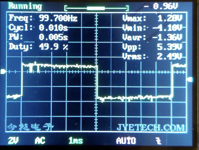
Yep, that is indeed a square wave. A noisy one at that, but considering it [the scope] is powered by a cheap wall-wart adapter it is OK. We can see that our signal is pretty close to 100Hz so that's another good sign.
Previously we say that plugging in a mere 100 nF cap didn't really change the shape much, but our sophisticated scope can actually pick uo the difference now; that is also nice.
Anyway.
A square wave can be thought as an infinite Fourier sum of its many (infinite) odd harmonics, so if we do a low-pass filter on the signal such that it is just enough to pass the carrier frequency ($f_c$) while damping ("attenuating") its harmonics ($3f_c$, $5f_c$, ...)
Desmos Square Wave Fourier Series, I didn't make this.
RC Low Pass filter
An RC low pass filter is exactly what it sounds like: Literally an RC circuit that is tuned with specific R and C values. All roads lead back to impedance. For high frequency, the cap in parallel acts like a short circuit (low impedance). The signal passes to ground through it instead of going down the path we are probing. For low frequency, it acts as a short circuit (high impedance) so current passes to the probed node. The effect is that low frequency components pass but high frequency components are blocked. Surprisingly simple but really useful.
The formula for an RC filter (both the low and high pass filter share the same math, just inverted topologies)
$$ f_c = \frac{1}{2\pi R C} $$
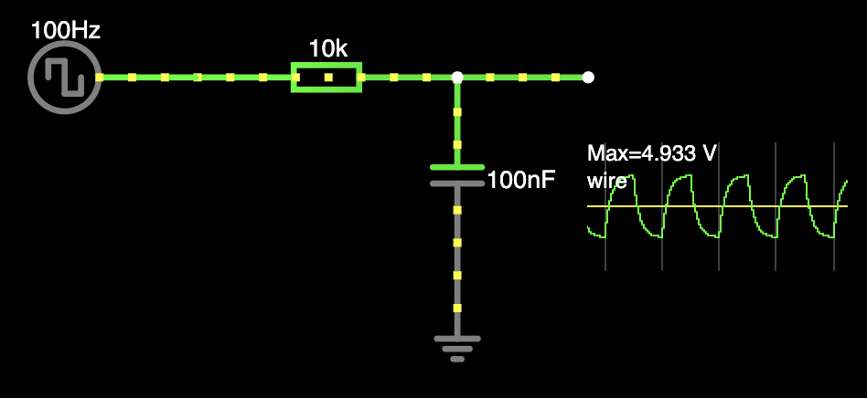
I chose an R value of 10k and C value of 100nF, which amount to a cutoff frequency of around 159Hz -- enough to pass $f_c$ but not $3f_c$ and beyond hopefully.
We only need to swap the 1k sense resistor for a 10k and just "test" a 100nF capacitor like we did previously, and, bam, low-pass filter. We techically had an RC low-pass filter all along now that I think about it, as this is an RC circuit anyway. Now it is tuned to reject anything above 160Hz.
Lo and behold...
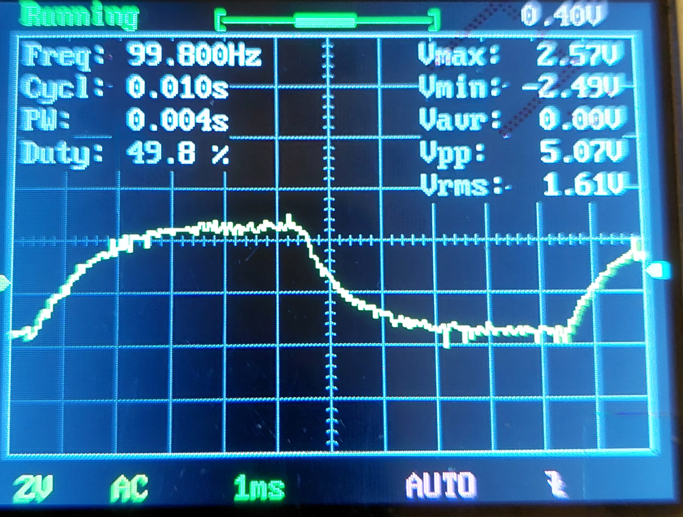
That... is not a sine wave at all. In fact it looks a lot like a regular RC cycle.
So turns out this RC filter is sort of weak. It is something called a first order filter, presumably because it has only one (1) reactive component. Those apparently "attenuate signals at a rate of $-20dB$ per decade.". This jargon means that 1) the unwanted harmonics don't get supressed as easily and 2) you actually can never fully block frequencies that don't clear the bar because attenuation is measured in decibels, a logarithmic scale. In fact here is an ideal simulation that shows the same RC "shark fin" characteristic:
We can make our filter girthier by increasing its order. Basically adding more resistors and capacitors and growing it like a tree. (but sideways instead of upside down) Each stage adds another "$-20dB$ per decade." attenuation.
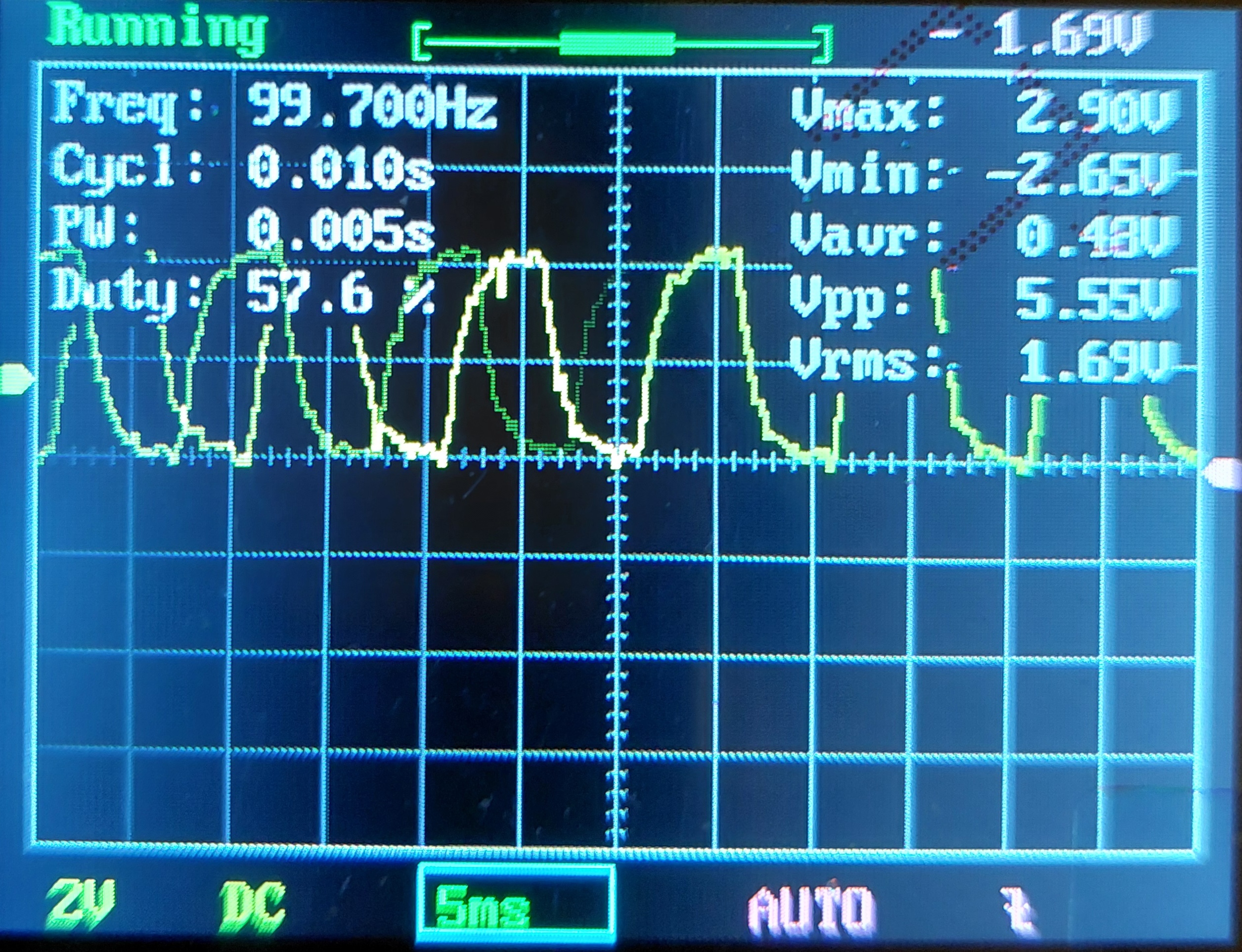
I added another R + C pass to the circuit and the signal looks slightly better now.
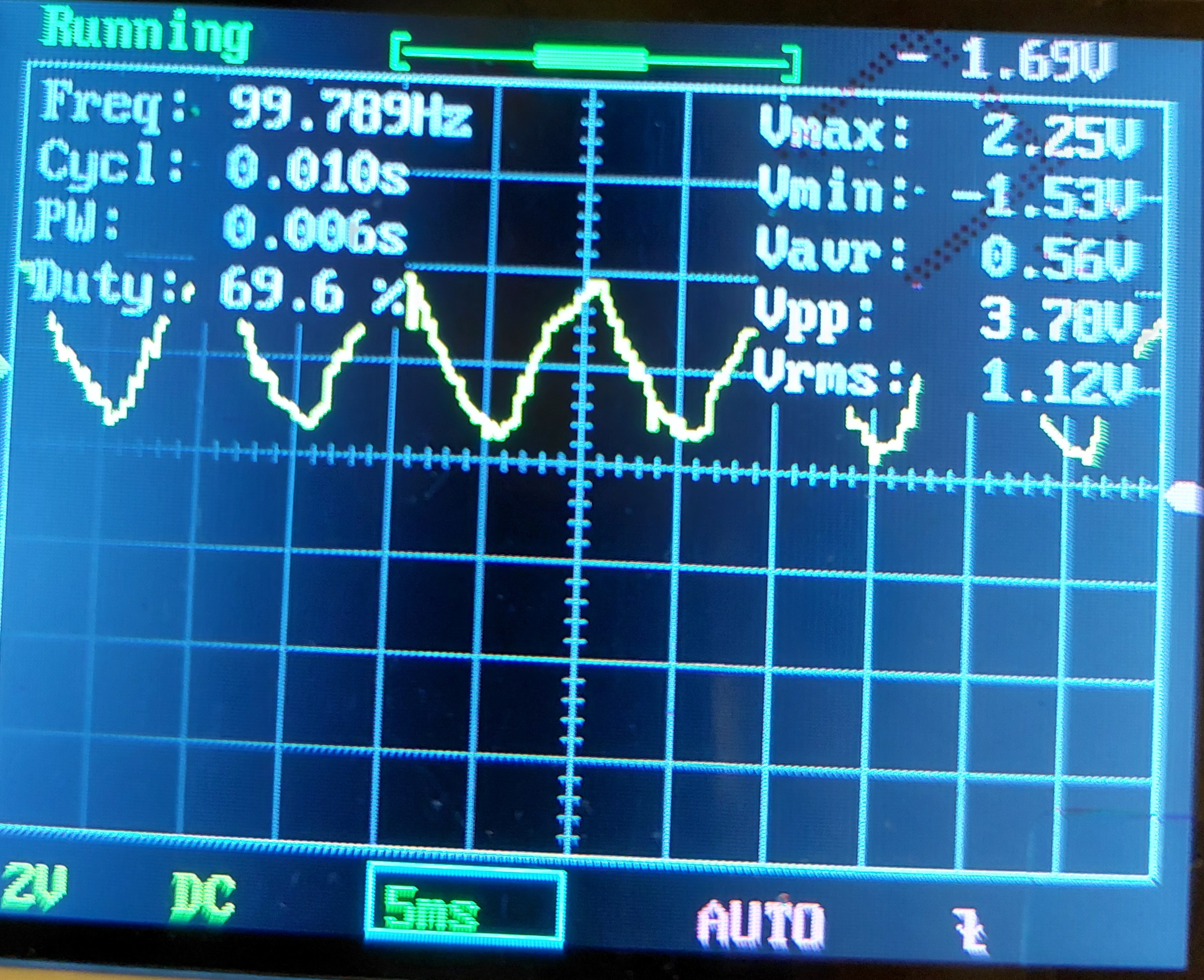
The keyword is better because it isn't remotely good, still looks a lot like a triangle wave because the cap is literally integrating our source signal (a square wave is the derivative of a triangle wave) as the cutoff frequency is considerably higher than the signal frequency. This is because the capacitances needed for a very-near 100Hz cutoff need to be really precise, and I cannot get that level of precision with my 104, 103, 102, etc. ceramics (I could put like 7 of them in parallel if I wanted to get really close but no). If I keep adding resistors and capacitors eventually the signal will look like a sine because of back-to-back integration but I don't want to bother.
However if we up the frequency to, for example, 1kHz like originally planned, we can attenuate much easier. This is because the frequencies of the harmonics will be more distant (1000Hz -> 3000Hz instead of 100Hz -> 300Hz)
The great thing is, we don't even have to change any of the circuitry!
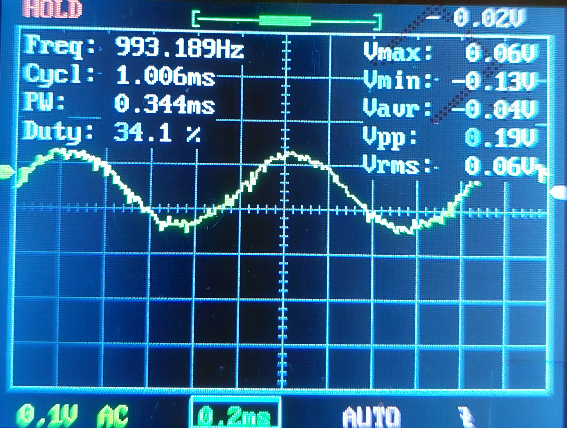
Details
There is another factor that contributes a lot to the sinusoidality (is that a word?) of the signal. You might be wondering how 10k + 100nF, which results in a cutoff frequency of 159Hz, is cleanly filtering a 1000Hz wave. The reason is that the cutoff frequency being below the signal frequency does not mean it gets deleted. The low pass is not a brick wall where all frequencies below its cutoff are immediately eliminated; just look at what we saw with the harmonics of 100Hz. It very well strongly diminishes the amplitude of the 1000kHz signal, but its harmonics even more so. If you look at the peak to peak voltage it isn't more than a measily 200mV by the time the signal reaches the scope.